
The particle trajectory function 'plotmass'
The function plotmass allows one to do a particle trajectory plot using Natural Coordinates, as defined by Allan Organ: 'Natural' coordinates for analysis of the practical Stirling cycle (ImechE, 1992). Refer also to Chapter 9 of his book: The Regenerator and the Stirling Engine (John Wiley, 1997).
Essentially, for an ideal gas the mass in any volume is inversely proportional to the temperature. Thus for the particle mass trajectory plot we normalize the volumes with respect to the local temperature. In the typical particle trajectory plot shown below the reduced volumes of the expansion and heater spaces are much smaller than those of the cooler and compression spaces. The regenerator is normalized with respect to the regenerator mean effective temperature.
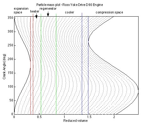 This
plot shows particles of equal mass flowing through the engine over a
cycle. In this design it appears as though the cooler volume can be
reduced, since some mass particles never leave the cooler. This
information is not intuitively obvious, and enables a better
understanding of the process, however at this stage it should not be
used to influence the design of the machine.
This
plot shows particles of equal mass flowing through the engine over a
cycle. In this design it appears as though the cooler volume can be
reduced, since some mass particles never leave the cooler. This
information is not intuitively obvious, and enables a better
understanding of the process, however at this stage it should not be
used to influence the design of the machine.
The following MATLAB function plotmass was developed by students of the Stirling Cycle Machine Analysis course, and is invoked by the function Schmidt .
   function


   plotmass


   % Kyle Wilson 10-2-02


   % Stirling Cycle Machine Analysis ME 589


   % Particle Trajectory Map


   % Equations from Organ's "'Natural' coordinates for analysis of the practical


   % Stirling cycle" and Oegik  Soegihardjo's 1993 project on the same topic


   % Modified by Israel Urieli (11/27/2010) to obtain correct phase advance


   % angle alpha subsequent to error determined by Zack Alexy (March 2010)


   % Global values from define program


   global


   vclc vcle


   % compression,expansion clearance vols [m^3]


   global


   vswc vswe


   % compression, expansion swept volumes [m^3]


   global


   alpha


   % phase angle advance of expansion space [radians]


   global


   vk


   % cooler void volume [m^3]


   global


   vh


   % heater void volume [m^3]


   global


   vr


   % regen void volume [m^3]


   global


   pmean


   % mean (charge) pressure [Pa]


   global


   tk tr th


   % cooler, regenerator, heater temperatures [K]


   NT = th/tk;


   % Temperature ratio


   Vref = vswe;


   % Reference volume (m^3)


   %% Fixed reduced volumes (dimensionless)


   vswe_r = (vswe/Vref)/NT;


   % Reduced expansion swept volume


   vcle_r = (vcle/Vref)/NT;


   % Reduced expansion clearance volume


   vh_r = (vh/Vref)/NT;


   % Reduced heater void volume


   vr_r = (vr/Vref)*log(NT)/(NT-1);


   % Reduced regenerator void volume


   vk_r = (vk/Vref);


   % Reduced cooler void volume


   vswc_r = (vswc/Vref);


   % Reduced compression swept volume


   vclc_r = (vclc/Vref);


   % Reduced compression clearance volume


   %% Phase domain


   angi = 0;


   angf = 2*pi;


   dang = 0.1;


   ang = [angi:dang:angf];


   n = size(ang);


   %% Reduced volume variations


   for


   i = 1:n(2)


   deg(i) = ang(i)*180/pi;


   Ve(i) = (vswe/2)*(1- cos(ang(i)));


   % Expansion volume vs phase


   Vc(i) = (vswc/2)*(1+ cos(ang(i) - alpha));


   % Compression volume vs phase


   ve(i) = (Ve(i)/Vref)/NT;


   % Reduced expansion vs phase


   vc(i) = Vc(i)/Vref;


   % Reduced compression vs phase


   vt(i) = vswe_r + vcle_r + vh_r + vr_r + vk_r + vclc_r + vc(i);


   % Total volume vs phase


   end


   figure


   step = 30;


   for


   m = 1:step-1


   for


   i = 1:n(2)


   v(i) = ve(i) + (m/step)*(vt(i)-ve(i));

   % Reduced volume segments


   end


   hold on


   plot(v,deg,


   'k:'


   )


   end


   hold on


   plot(ve,deg,


   'k'


   )


   plot(vt,deg,


   'k'


   )


   %% Vertical lines


   L1 = vswe_r;


   % Boundary of reduced expansion swept volume


   L2 = L1 + vcle_r;


   % Boundary of reduced expansion clearance volume


   L3 = L2 + vh_r;


   % Boundary of reduced heater void volume


   L4 = L3 + vr_r;


   % Boundary of reduced regenerator void volume


   L5 = L4 + vk_r;


   % Boundary of reduced cooler void volume


   L6 = min(vt);


   % Boundary of reduced expansion swept volume


   point1 = [L1;L1];


   % Preparing for plot


   point2 = [L2;L2];


   point3 = [L3;L3];


   point4 = [L4;L4];


   point5 = [L5;L5];


   point6 = [L6;L6];


   point = [0;deg(n(2))];


   plot(point1, point,


   'r--'


   , point2, point,


   'r--'


   , point3, point,


   'g--'


   )


   plot(point4, point,


   'g--'


   , point5, point,


   'b--'


   , point6, point,


   'b--'


   )


   axis([0 max(vt) 0 deg(n(2))])


   xlabel(


   'Reduced volume'


   )


   ylabel(


   'Crank Angle (deg)'


   )


   title(


   'Particle mass plot'


   )


   hold off

Stirling Cycle Machine Analysis
by Israel
Urieli
is licensed under a Creative
Commons Attribution-Noncommercial-Share Alike 3.0 United States
License