MATLAB program for plotting a Simplified Psychrometric Chart ( Updated 3/7/08 )

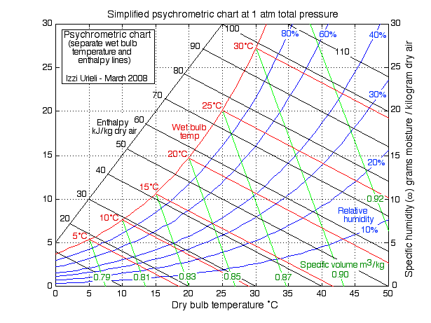
The MATLAB program ( psychro.m ) (shown below) is used to plot the Simplified Psychrometric Chart shown above. Data is read from 2 datafiles containing water saturation temperature/pressure data, file t_pg over 1°C intervals for plotting the saturation and constant relative humidity curves, and file t_pg1 over 5°C intervals for plotting the wet-bulb temperature and enthalpy lines. The source of the data: NIST Chemistry WebBook - accessed Feb 2008

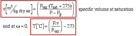
The following four equations (refer back to Part 1 and Part 2 ) are evaluated in the program:

specific humidity: (sometimes known as: humidity ratio or absolute humidity):
:

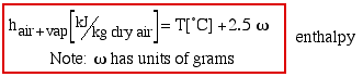
Notice in the psychrometric chart that the oblique enthalpy axis is given by= T+5, for T varying between 0°C to 25°C. Substituting this value ofin the enthalpy equation (above) leads to the intercept of the enthalpy line with the enthalpy axis as follows:

h = T + 2.5 (T + 5)

or finally: T = (h - 12.5)/3.5

Thus the enthalpy lines can be plotted parallel to, but independant of the wet bulb temperature lines.

The complete MATLAB program follows. Note that it is the convention in programming that all variable names begin with lower case letters. Thus t represents temperature [°C], p represents pressure [kPa], w (in place of) represents specific humidity [grams / kg dry air] (aka: absolute humidity, humidity ratio), h represents enthalpy (kJ/kg dry air) and the suffix g represents the saturated vapor state (following the convention used in steam tables).

   % Plotting the Simplified Psychrometric Chart 
 
 
   % Izzi Urieli 2/27/2008 
 
 
   tpg = dlmread( 
 
  't_pg' 
 
  , 
 
  '\t' 
 
  ); 
 
  % saturation temp/pressure 
 
 
   t = tpg(:,1); 
 
  % temperature (C) 
 
 
   pg = tpg(:,2); 
 
  % saturation vapor pressure (kPa) 
 
 
   patm = 101.325; 
 
  % standard atmosphere (kPa) 
 
 
   rair = 0.287; 
 
  % gas constant of air (kJ/kg.K) 
 
 
   wg = 622*pg./(patm-pg); 
 
  % saturation specific humidity 
 
 
   plot(t,wg, 
 
  'r-' 
 
  ) 
 
 
   hold 
 
 
   grid 
 
 
   for 
 
  phi = 0.1:0.1:0.4, 
 
  % phi = relative humidity 10% - 40% 
 
 
   w = 622*phi*pg./(patm-phi*pg); 
 
 
   plot(t,w) 
 
 
   end 
 
 
   for 
 
  phi = 0.6:0.2:0.8, 
 
  % phi = 60%, 80% 
 
 
   w = 622*phi*pg./(patm-phi*pg); 
 
 
   plot(t,w) 
 
 
   end 
 
 
   % specific volume and enthalpy/wet-bulb-temp 
 
 
   tpg1 = dlmread( 
 
  't_pg1' 
 
  , 
 
  '\t' 
 
  ); 
 
 
   t1 = tpg1(:,1); 
 
  % saturation temperature (C) 
 
 
   pg1 = tpg1(:,2); 
 
  % saturation pressure (kPa) 
 
 
   wg1 = 622*pg1./(patm-pg1); 
 
  % saturation specific humidity 
 
 
   % specific volume of dry air (cubic m/kg dry air) (green) 
 
 
   vol = rair.*(t1+273)./(patm-pg1) 
 
  % specific vol at saturation 
 
 
   tv0 = patm*vol/rair-273; 
 
  % air temperature at zero humidity 
 
 
   for 
 
  i = 1:7, 
 
 
   plot([t1(i),tv0(i)],[wg1(i),0], 
 
 
   'g-' 
 
 
   ) 
 
 
   end 
 
 
   % wet bulb temperature (also enthalpy) lines (red) 
 
 
   h = t1 + 2.5*wg1 
 
  % enthalpy (kJ/kg-dry-air) (displayed) 
 
 
   t0 = h; 
 
  % temperature at zero humidity for enthalpy h 
 
 
   for 
 
  i = 1:6, 
 
 
   plot([t1(i),t0(i)],[wg1(i),0], 
 
 
   'r-' 
 
 
   ) 
 
 
   end 
 
 
   % enthalpy axis and enthalpy lines (black) 
 
 
   for 
 
  h = 10:10:110, 
 
  % enthalpy (kJ/kg-dry-air) 
 
 
   t0 = h; 
 
 
   % temperature at zero humidity 
 
 
   t1 = (h - 12.5)/3.5; 
 
 
   % temperature on the enthalpy axis 
 
 
   w1 = t1 + 5; 
 
 
   % specific humidity on the enthalpy axis 
 
 
   plot([t0,t1],[0,w1], 
 
 
   'k-' 
 
 
   ) 
 
 
   end 
 
 
   plot([0,25],[5,30], 
 
  'k-' 
 
  ) 
 
  % the oblique enthalpy axis 
 
 
   axis([0,50,0,30]) 
 
  % limit the range of the chart 
 
 
  title( 
  'Simplified Psychrometric Chart' 
 
 ) 
 
  xlabel( 
  'Dry Bulb Temperature (deg C)' 
 
 ) 
 
  ylabel( 
  'Specific Humidity (gm vap/kg dry air)' 
 
 ) 
 

Notice in the program that both the specific volume (vol) and the enthalpy values (h) are displayed (no semicolon) thus they can be subsequently added to the plot together with the relevant saturation/wet bulb temperatures. relative humidity values.and enthalpy values on the enthalpy axis.